

Discounted Cash Flow
What is covered
A discounted cash flow (DCF) analysis is one of the most fundamental valuation methods in finance. It is used to estimate the intrinsic value of a business by projecting its future cash flows and discounting them back to today at a rate that reflects risk. Rather than relying on market sentiment or comparable companies, a DCF focuses on the underlying economics of a business, including its growth, profitability, and capital requirements. This framework is widely used in investment banking, private equity, corporate finance, and investing to evaluate acquisitions, investments, and strategic decisions, making it a cornerstone of financial analysis.
What is a DCF model?
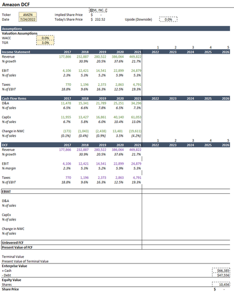
A DCF, like it says in the intro, is a way to come to a value estimate for something through predictions and opinions that an analyst makes. Below is the answer to a "Walk me through a DCF," interview question, and after that we go through each part with excel examples and walkthroughs. The picture to the right is an incomplete DCF and by the time we finish this model at the bottom the DCF and all of its parts will be filled in.
"Can you walk me through a DCF?"
"To perform a (DCF) valuation, you first project a company’s revenue, operating expenses, taxes, and repeatable cash flow items, such as depreciation and amortization, capital expenditures, and changes in net working capital. These projections are used to calculate free cash flow over a forecast period, typically spanning five to ten years. Once the free cash flows are projected, they must be discounted back to their present value using a discount rate known as the weighted average cost of capital, or WACC. This rate reflects the return investors expect for putting money into the company and accounts for both the cost of equity and the cost of debt.
After discounting each year’s projected free cash flow, we sum them to get the present value of the forecasted period. However, a business hopefully doesn't stop operating after the projected years, so we need to estimate the value of all future cash flows beyond that point. This is done by calculating a terminal value. There are two main methods to determine terminal value. The first is the Gordon Growth Method, which assumes that cash flows will continue to grow indefinitely at a modest, stable rate, such as GDP. The second is the Exit Multiple Method, which estimates the company’s value based on a multiple of its financial metric, such as EBITDA, at the end of the forecast period.
Once the terminal value is calculated, it too is discounted back to present value using the WACC. The final step in the DCF process is to add the present value of the forecasted free cash flows to the discounted terminal value. This total gives the implied enterprise value of the company. Then take the EV and add cash and subtract debt to get equity value."
PT 1 - Projecting Free cash flow
A DCF begins with projecting unlevered free cash flow, which represents the cash a business generates from operations after reinvesting in itself, but before considering how it is financed. This allows the valuation to remain independent of capital structure. The formula begins with NOPAT or EBIT*(1 - tax rate) as these are the same
NOPAT or EBIT* (1 - tax rate) + depreciation and amortization - capital expenses + change in net working capital
Income Statement
The projected years for this model are 2022 - 2026. The process starts with income statement assumptions, which are typically driven by growth rates based on historical performance, management guidance, or industry expectations. This begins with revenue projections for each forecast year, then operating costs are modeled, and this is used to arrive at operating income (EBIT).

Taxes are then taken out because unlevered free cash flow begins with NOPAT (Net operating profit after taxes) which is the same as EBIT - taxes or EBIT*(1 - tax rate). Importantly, taxes are calculated as if the company has no debt, meaning interest expense is ignored at this stage. This preserves the “unlevered” nature of the cash flow.
PT 2 - Projecting the Cash flow statement
Once the income statement items are projected, you have to project the cash flow statement. From the cash flow statement, you get depreciation and amortization (D&A), capital expenses (Capex), and the change in net working capital (Change in NWC). These are projected the same way as the income statement items, through market predictions, analyst opinions on the company's future, and how much they think the company will spend on infrastructure/expansion in the next 3-7 years.

By taking the revenue and then EBIT as a percent margin (56,145 is 9.4% of 594,752) this gets you to your operating income (EBIT). This is calculated through, like we just went through, projections from your income statement. Then by either adding taxes (EBIT + Taxes) or multiplying EBIT by 1 - tax rate you arrive at NOPAT (EBIAT or earnings before interest after taxes).

This is where the formula we went over at the top comes into play:
NOPAT or EBIT* (1 - tax rate) + depreciation and amortization - capital expenses + change in net working capital

By starting with EBIAT + D&A - CapEx + change in NWC = Unlevered free cash flow. Now the problem is that a dollar today is worth more than a dollar tomorrow. This is in part due to inflation but mainly has to do with the concept of investing. If you stick 100 under a mattress for 1 year is will still be 100 dollars in 1 year. But if you take that 100 dollars and put it into a money market at 4%, then at the end of the year it is at 104 dollars. So, since a dollar today is worth more than a dollar tomorrow because we can invest that dollar and earn a return, this difference needs to be accounted for. As the 190,641 listed in year 5 for EBIAT is not worth 190,641 when that time comes it, it will be worth something less. So, using the formula FCF / (1 + WACC) ^ the year, we can account for that difference. So, if it is 2026 you would raise it to the power of 5, because the end of 2026 is 5 years from the start of 2022.
PT 3 - Discount rate (WACC)
This requires discounting those free cash flows back to what they would be worth today. To do this, we use the weighted average cost of capital. The WACC represents the average return a company must generate to satisfy all of its capital providers, including equity holders and debt holders. It is used as the discount rate in a DCF because it reflects the risk of the company’s unlevered cash flows.
WACC is calculated by weighting the cost of equity and the after-tax cost of debt based on the company’s capital structure. The cost of equity is typically estimated using the Capital Asset Pricing Model (CAPM), which incorporates the risk-free rate, the company’s beta, and the equity risk premium. The cost of debt is based on the company’s borrowing rate and is adjusted for taxes to reflect the interest tax shield.
Because WACC captures both business risk and capital structure, it links a company’s operating performance to its valuation. Higher risk results in a higher WACC and lower valuation, while lower risk leads to a lower WACC and higher valuation. We will go over all of this down below using the same excel model.
WACC Formula:
% of debt * cost of debt * (1 - Tax rate) + % of equity * cost of equity
If there is preferred equity than add in + % of pref equity * cost of pref equity to the end of the formula.
The cost of equity formula is essentially the same meaning as the WACC formula but only takes into account the cost for equity. How much the equity investors need to make to make their investment worth it without putting their money somewhere else.
The equation for the cost of equity is:
Risk free rate + Beta * Market risk premium
All of these things are gone over in the technical guide in interview prep in more detail.

PT 4 - Calculating Terminal Value
Because companies are assumed to continue operating beyond the explicit forecast period (3-10 years), a terminal value is used to capture the value of all future cash flows after the final projected year. The most common approach is the perpetual growth method, which assumes free cash flow grows at a stable, constant rate forever. The terminal value is calculated using the final year’s unlevered free cash flow, grown by a modest perpetual growth rate that typically reflects long-term economic growth (Normally the GDP os the economy as a company cannot grow at higher rates than the economy forever).
This terminal value is calculated as of the last forecast year, meaning it represents a future value. As a result, it must later be discounted back to today just like the annual cash flows. In most DCFs, the terminal value makes up a significant portion of the total enterprise value, which makes conservative assumptions critical.

Terminal Value formula: Final years FCF * (1 + terminal growth rate) / (WACC - TGR)
74,257 * (1 + 3.0%) / (7.82% - 3.0%)
Present value of terminal value formula: Terminal value / (1+WACC)^the amount of years projected out:
1,088,853 / (1 + WACC)^5
With unlevered free cash flows, terminal value, and WACC calculated, the next step is to determine enterprise value. Each year’s free cash flow is discounted back to present value using WACC, and the present value of the terminal value is added to the sum of discounted cash flows.
This total represents the value of the company’s core operations, or enterprise value. To arrive at equity value, non-operating items are then accounted for. Cash and cash equivalents are added, while debt, preferred equity, and other claims senior to common equity are subtracted. The result is total equity value. If the goal is to estimate a per-share value, equity value is divided by diluted shares outstanding, yielding an implied intrinsic share price.
Enterprise value formula:
Present value of terminal cash flow + Sum of present values of future cash flows = EV
747,241 + 40,215 + 48,662 + 58,451 + 52,855 + 50,960 = 1,017,214
EV + cash - debt = Equity value
Equity value / diluted shares outstanding = estimated share price

A DCF is built sequentially, with each section feeding directly into the next. Operating assumptions drive unlevered free cash flow. Free cash flow feeds terminal value. Both are discounted using WACC to calculate enterprise value, which is then bridged to equity value. When structured clearly in Excel, this flow allows assumptions to be adjusted easily and makes the valuation transparent, logical, and defensible.
Complete DCF model with estimated share price:


A DCF analysis is most commonly used in industries with relatively predictable and cash-generative business models, where future performance can be reasonably forecasted. This includes sectors such as industrials, consumer staples, mature healthcare and technology companies, energy, infrastructure, and utilities. Companies in these industries often have established operating histories, stable demand drivers, and identifiable capital spending needs, which make cash flow projections more reliable. Across these sectors, a DCF is used to evaluate investments, acquisitions, capital projects, and strategic decisions by focusing on the long-term ability of a business to generate cash rather than short-term market movements.